What phase disorder does to the GHZ advantage

23 September 2026

An entangled array of \(N\) qubit sensors can reach the Heisenberg limit: a quantum Fisher information (QFI) of \(N^2\) for a signal that every sensor sees the same way, against \(N\) for independent sensors. For an AC field that assumption is easy to break. The field reaches different sensors with different phases \(\phi_i\), so after demodulation sensor \(i\) picks up the signal \(\theta\) with a coupling \(g_i = \cos\phi_i\) that can be small or even negative.

I wanted to know how much of the advantage survives. To find out I used squint, Benjamin MacLellan’s JAX framework for differentiable quantum metrology.

One Fisher matrix instead of many simulations

squint differentiates a circuit with respect to whichever parameters you mark. I put one \(R_z\) gate per sensor into a single Block, so one call returns the \(N \times N\) QFI matrix over the local phases:

phases = Block()
for w in wires:
    phases.add(RZGate(wires=(w,), phi=0.1))
circuit.add(phases, "phases")

params, static = partition_op(circuit, "phases")
sim = Simulator(static=static, params=params)
F = quantum_fisher_information_matrix(sim.forward, sim.grad, params)

The structure of \(F\) already tells the story. For the product state \(|{+}\rangle^{\otimes N}\) it is the identity. For the GHZ state it is the all-ones matrix: the state only responds to the sum of the phases. For any couplings the chain rule gives

\[ F_\theta = g^{\mathsf T} F\, g , \]

so averaging over thousands of random phase patterns is a quadratic form, not thousands of simulations. Measuring every qubit in the \(X\) basis reaches this bound: squint’s classical Fisher information for that readout equals \(F\).

What the disorder does

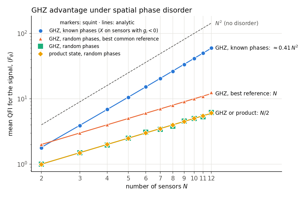
Mean QFI versus number of sensors for four strategies

With uniformly random phases:

GHZ: \((\sum_i \cos\phi_i)^2\) averages \(N/2\), exactly the same as the product state. The entanglement buys nothing.
GHZ with the best common reference phase for the control sequence: \(|\sum_i e^{i\phi_i}|^2\), which averages \(N\). That is back at the standard quantum limit, not beyond it.
GHZ with known phases: apply \(X\) to every sensor with \(\cos\phi_i < 0\) right after preparing the GHZ state. That flips the sign of its phase, all the contributions add up, and the mean QFI becomes \((2/\pi)^2 N^2 \approx 0.41\,N^2\). Heisenberg scaling comes back at 41% of the ideal, for the price of a few single-qubit gates.

The markers are squint and the lines are the analytic averages; they agree for \(N = 2\) to \(12\).

squint makes three extensions easy, and I want to try them: dephasing during the sensing time, which limits how large a compensated GHZ state is still worth preparing; a photonic version in which the sensors are optical modes; and optimizing the preparation circuit end to end instead of fixing it, as in the variational sensing work behind squint.

The code is qsensing.fisher and qsensing.disorder in my Quantum-Sensing repository.

What phase disorder does to the GHZ advantage

One Fisher matrix instead of many simulations

What the disorder does

Next