Expressive is not the same as learnable
24 September 2026
At the ML4QT meeting at IQC this week, one talk laid out what machine learning is used for in quantum physics: predicting properties of a state from measurement data, reconstructing the distribution of measurement outcomes, and training variational models on a Hamiltonian. It gave me better vocabulary for my master’s thesis than the one I wrote it in, so this post goes through the thesis again using that map.
The short version: I trained four kinds of model on the same one-dimensional rotated cluster state. The state is an exact matrix product state (MPS) with bond dimension 2 at every length and angle, so for the complex variational models capacity was never the problem. The clearest difference between the models was whether their internal update already had the shape of that two-dimensional memory.
The test state
Start from the 1D cluster state and rotate every qubit by \(R_y(\theta)\). A local rotation cannot change the Schmidt rank across any cut, so the exact bond dimension stays \(D = 2\). The measured outcomes are a different story. I measure how long they stay dependent with the conditional mutual information (CMI) between the two ends of a buffer of \(m\) sites,
In the entanglement-swapping readout, where the bulk stabilizers are \(X_{j-1}Z_jX_{j+1}\), the endpoint CMI is exactly one bit at \(\theta = 0\): the parity of the two endpoint bits is fixed by a parity of the middle outcomes. At \(\theta = \pi/2\) it is zero. The previous post looked at the conventional readout of the same state.
So the state has a small memory that can live for a long time. That makes it a controlled test for neural quantum states: since the target is known to fit in a bond of dimension 2, any difficulty a model has must come from optimization, sampling or how it is parameterized.
Linear and nonlinear properties
The talk sorted the properties we want from a quantum system into linear ones, \(\mathrm{Tr}(\rho O)\), such as magnetization, two-point correlations and order parameters, and nonlinear ones such as purity, entanglement entropy and mutual information. The rotated cluster state shows why the split matters.
A local basis rotation changes the matrix that each individual outcome applies to the bond, but it leaves the outcome-averaged transfer channel \(\mathcal{E}(X) = \sum_x A^x X A^{x\dagger}\) unchanged. For the cluster tensor this channel has spectrum \(\{1, 0, 0, 0\}\), so ordinary two-point correlations are gone after at most two sites, at every angle. The CMI conditions on a particular measurement record instead of averaging over records, and it moves from one bit to zero as \(\theta\) goes from \(0\) to \(\pi/2\). Ordinary two-point correlations stay short-ranged at every angle while the CMI changes completely.
An exact control: the AKLT chain
Before trusting the CMI code on the cluster state I wanted a case where the answer is known in closed form. The spin-1 AKLT chain is also a bond-dimension-2 MPS, and it can be solved by sorting each measurement outcome by what it does to the virtual bond.
- Outcomes \(+\) and \(-\) select rank-one matrices. Whatever virtual state comes in, the same one goes out, so the memory is reset.
- Outcome \(0\) is proportional to \(\sigma^z\), a unitary. It keeps the memory, up to a known Pauli byproduct, and it occurs with probability 1/3.
Information about the left endpoint survives a buffer of \(m\) sites only if all \(m\) outcomes are \(0\), which has probability \(3^{-m}\). Two adjacent outcomes share \(4/9\) bits, so
This equals the ordinary correlation length, since the transfer spectrum is \(\{1, -1/3, -1/3, -1/3\}\). The equality is special to this model: the same 1/3 is both the magnitude of the subleading eigenvalue and the probability of the only outcome that keeps the memory. My exact MPS contractions reproduce the formula to numerical precision, which is how I checked the CMI code.
The same keep-or-reset view explains the cluster state. In the entanglement-swapping frame a representative bulk outcome acts on the bond as
with singular values \(\tfrac{1}{\sqrt 2}\lvert\cos\tfrac{\theta}{2} \pm \sin\tfrac{\theta}{2}\rvert\). At \(\theta = 0\) they are equal and the map is a unitary that keeps both directions of the bond. At \(\theta = \pi/2\) one of them is zero and the map is a reset. In between, every outcome partly filters the bond, and \(\lvert\det B\rvert = \tfrac12\lvert\cos\theta\rvert\) is the same factor that appears in the known upper bound \(I_m \le \lvert\cos\theta\rvert^m\).
The picture I ended up with is that memory size, memory lifetime and readout are three different things. The bond dimension fixes the first, the rotation angle sets the second, and the choice of measurement decides whether the surviving information is visible at all.
Building the memory into the model
An MPS can be read as a recurrent network. After \(j\) sites the contraction has produced a bond vector \(h_j\), and the next measurement outcome selects the matrix that updates it:
I turned this into a trainable model with three design choices.
- The hidden state is the bond vector. The model knows that its memory is a \(\chi\)-dimensional complex vector updated by a matrix that depends on the outcome. It still has to learn what those matrices are.
- Separate tensors for even and odd sites. In the entanglement-swapping representation, neighbouring sites act on the bond in alternating ways, one X-like and one Z-like. Two bulk tensors \(A_{\mathrm{even}}\) and \(A_{\mathrm{odd}}\), which \(\pi(j)\) picks between, let the update alternate between the two sublattices without fixing either tensor to its exact value. With boundary tensors \(L\) and \(R\) the model has \(8\chi + 8\chi^2\) real parameters, which is 48 at \(\chi = 2\).
- A capacity control. The same model at \(\chi = 1\) has 16 parameters and is a product state. It cannot carry a virtual parity, so comparing it with \(\chi = 2\) changes only the size of the memory.
I trained it at \(N = 64\) and \(\theta = 0.35\), an angle where the endpoint memory is long but finite.
- The energy is computed exactly by contracting the network, reusing prefix and suffix environments, so each evaluation costs \(O(N)\) and there is no Monte Carlo noise in the gradient.
- The two bulk tensors have a gauge freedom: \(A_{\mathrm{even}} \to cA_{\mathrm{even}}\) together with \(A_{\mathrm{odd}} \to c^{-1}A_{\mathrm{odd}}\) leaves the wavefunction unchanged, so the raw parameters can drift to very different scales. Rescaling the Frobenius norm of each tensor group after every Adam step made the optimization much more stable.
- 150 Adam steps from random complex initial tensors find the right basin, with total energy errors between \(1.2\times10^{-5}\) and \(2.8\times10^{-4}\). Up to 50 L-BFGS iterations then refine it.
All five random initializations reached the ground state. The median total error is \(E - E_0 = 9.98\times10^{-12}\), an energy-density error of \(1.56\times10^{-13}\). Because the Hamiltonian is a sum of commuting stabilizers, I also checked every term separately: the smallest \(\langle K_j\rangle\) over all sites and seeds is 0.999999999956, so the low energy is not the result of local errors cancelling. The \(\chi = 1\) control stays at \(E - E_0 = 32\) with average stabilizer value 1/2. The optimizer works; the product state has no room for the memory.
The generic learners
The same state, with three generic models that each answer a different question:
| Model | Trained on | Size, angle | Result |
|---|---|---|---|
| Complex RBM, 592 parameters | exact energy, summed over all basis states | \(N = 8\), \(\theta = 0\) | median energy-density error \(6.03\times10^{-8}\) (5 seeds) |
| GRU, hidden size 16 | 8192 measured bitstrings | \(N = 64\), \(\theta = 0.35\) | median KL divergence \(3.7\times10^{-3}\) bits/site, classical fidelity 0.898 (3 seeds) |
| tanh RNN, VMC | sampled local energies | \(N = 64\), \(\theta = 0.35\) | best of four runs \(E - E_0 \approx 0.57\); all still falling when a time limit stopped them |
| MPS-induced, \(\chi = 2\), 48 parameters | exact energy | \(N = 64\), \(\theta = 0.35\) | median energy-density error \(1.56\times10^{-13}\) (5 seeds) |
The RBM shows that a generic complex network can represent the state: at \(N = 8\), with no sampling, it gets there. Exact summation grows as \(2^N\), though, so this is a check of representation, not a result about large systems.
The GRU is the generative setting from the talk, implicit state reconstruction: learn a model \(Q_\theta\) of the measurement outcomes so that \(Q_\theta \approx P\). Going from 512 to 8192 training strings lowered the KL divergence from \(4.6\times10^{-2}\) to \(3.7\times10^{-3}\) bits per site and the error in the next-bit probability from 0.108 to 0.011. A 16-dimensional hidden state is enough to learn this long-memory distribution at \(N = 64\), given enough data.
The generic variational RNN is where the difference shows. It has to find a useful hidden coordinate, an update rule and the phase structure from noisy sampled gradients. Changing the learning rate did not change that, and in one short run doubling the hidden width from 64 to 128 did not clearly help either.
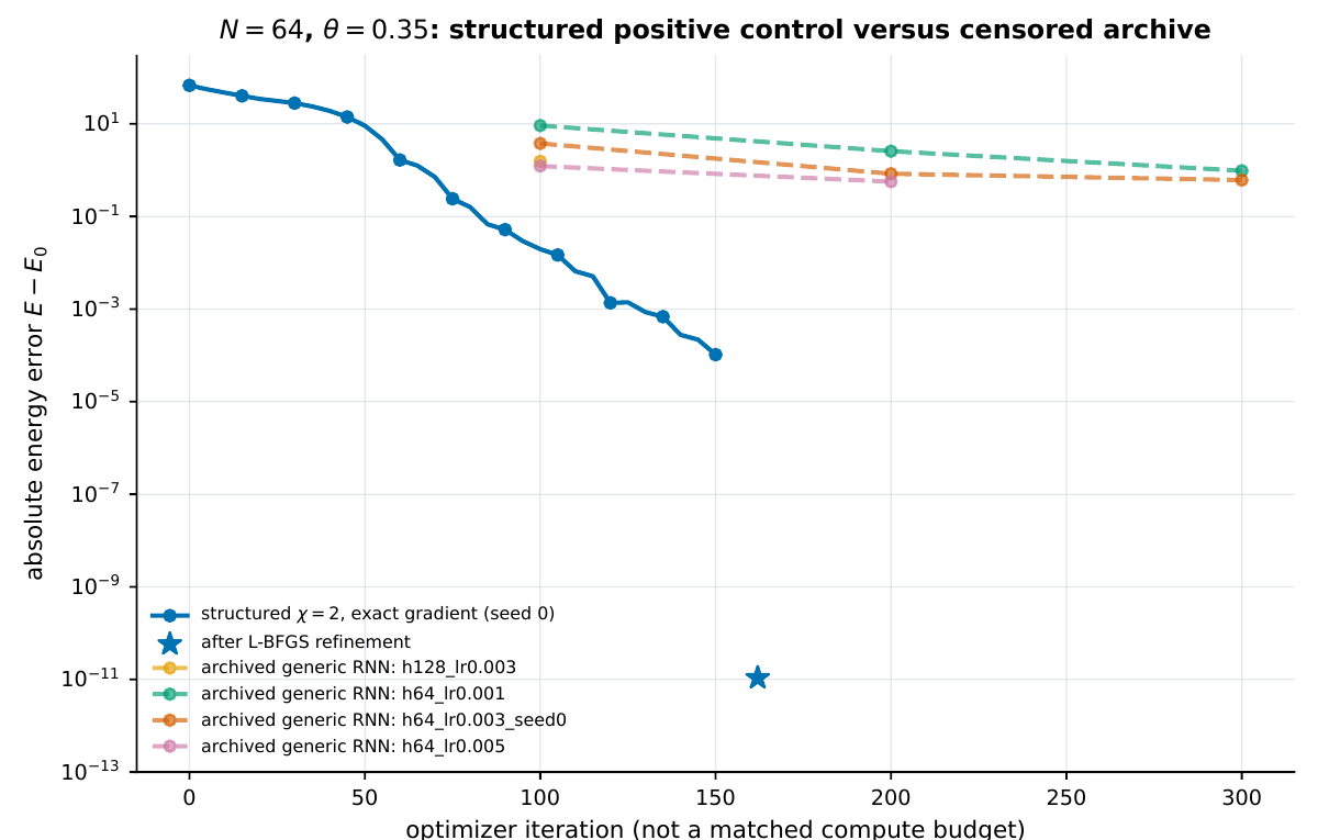
\(N = 64\), \(\theta = 0.35\). Solid line: one \(\chi = 2\) MPS-induced run with exact gradients; the star is the result after L-BFGS. Dashed lines: generic recurrent VMC runs. Iteration counts are not matched compute.
Three caveats. The VMC runs were stopped by a queue time limit, not by convergence, so they show slow progress rather than a final error floor. They also used sampled gradients while the MPS-induced model used exact ones, so this is a pilot comparison, not a matched one. And the \(\chi = 2\) model is matched to a state that is known to have bond dimension 2, so the comparison measures the value of a correct inductive bias, not a general advantage of MPS over neural networks.
The talk also covered neural scaling laws: performance that improves predictably with model size, data and compute. The GRU improved steadily as the training set grew. For the variational problem, though, a wider generic network did not clearly help in the one run I had, while a 48-parameter model with the right structure got to near machine precision.
What single-basis data cannot see
In generative reconstruction the model learns \(P(i) = \mathrm{Tr}(\rho\,\lvert i\rangle\langle i\rvert)\), only the diagonal of the density matrix in one basis. The GRU learns \(\lvert\psi(x)\rvert^2\) and nothing about relative phases. To make that concrete, at \(N = 8\) I measured the two endpoints in the \(Z\) basis and the middle pairs (2,3), (4,5) and (6,7) in the Bell basis. As a control I replaced every amplitude by its magnitude, \(\psi(x) \to \lvert\psi(x)\rvert\). The control has exactly the same \(Z\)-basis distribution, but the Bell readout sees a different CMI.
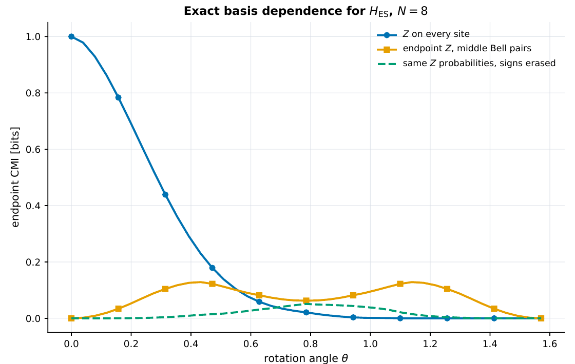
Exact \(N = 8\) results for the rotated entanglement-swapping state. Erasing the signs leaves the \(Z\)-basis distribution unchanged but changes what a Bell readout sees.
Any generative model trained in a single basis will fail this test by construction. The next experiment on the data side is to train on several bases and test on the Bell readout.
What I take from it
- Expressive and learnable are different questions. The complex variational models could all represent this state in principle. The one that learned it fast and reliably had a hidden update with the right shape built in: the right memory dimension, an outcome-dependent linear update, and the even/odd sublattice structure. Only the memory dimension was tested on its own, through the \(\chi = 1\) control. Separating the effect of the other two needs an ablation I haven’t run yet, such as a single shared bulk tensor instead of the even/odd pair.
- The design rule I would reuse: build in what you already know about the memory, and spend the learning capacity on what you don’t know.
- One slide was about provable learning advantages, where restrictions on the family of Hamiltonians, such as sparse or gapped local ones, make learning efficient. My results are numerical and about one family of states, not a theorem, but they point the same way from the model side: restricting the model class to the right structure made the optimization easy.
- The advantage is large here because the built-in structure is exactly right. The more interesting question is how it degrades when it is not. Adding a transverse field, or moving across the cluster-Ising phase diagram that another slide showed being mapped with tensorial-kernel support vector machines, would push the required bond dimension above the built-in one.
The exact MPS code for the CMI calculations is in my nqs_project repository.